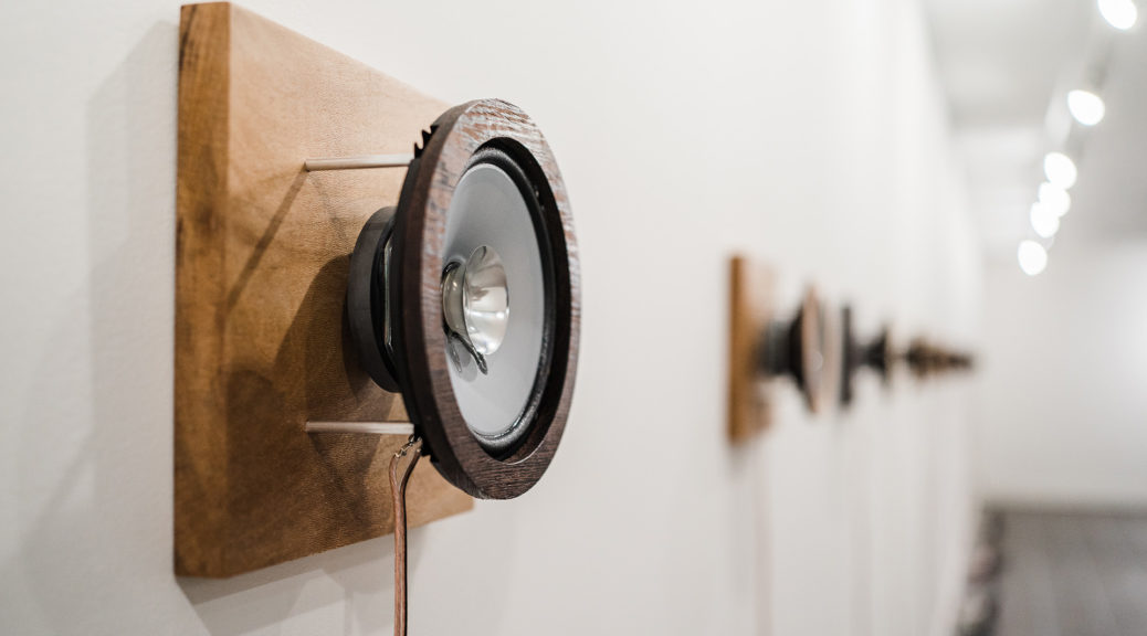
Wildfire is a 48-foot long speaker array that plays back a wave of fire sounds across its 48-foot span at speeds of actual wildfires. The sound art installation strives to have viewers embody the devastating spread of wildfires through an auditory experience.
Wildfire employs sound to investigate how the climate enables destructive wildfires that lead to statewide emergencies. The speed at which fires move can be mimicked in sound. By placing speakers along a surface (every three feet across 48 feet ~16 speakers), Wildfire implements spatialization techniques to play waves of fire sounds at speeds of simulated models and actual wildfire events. Comparing the speed of different fires through sound spatialization, we can hear how quickly different fires move across various wildfire behavior (fuel, topography, and weather).
Stereo audio example. Fire sound moving across stereophonic field at 16 mph.
Stereo audio example. Fire sound moving across stereophonic field at 83 mph.
Wildfire is comprised of sixteen 30W speakers, 120’ speaker cable, sixteen 8” square wood mounts, sixteen 6.25” diameter wood speaker rings, 64 aluminum speaker post mounts, eight custom electronic boards and enclosures, eight 50W power amps, one custom motherboard and enclosure, eight custom length Ethernet cables, custom-built power supply cable, sixteen 15V 4A power supplies, and three 9V 5A power supplies.
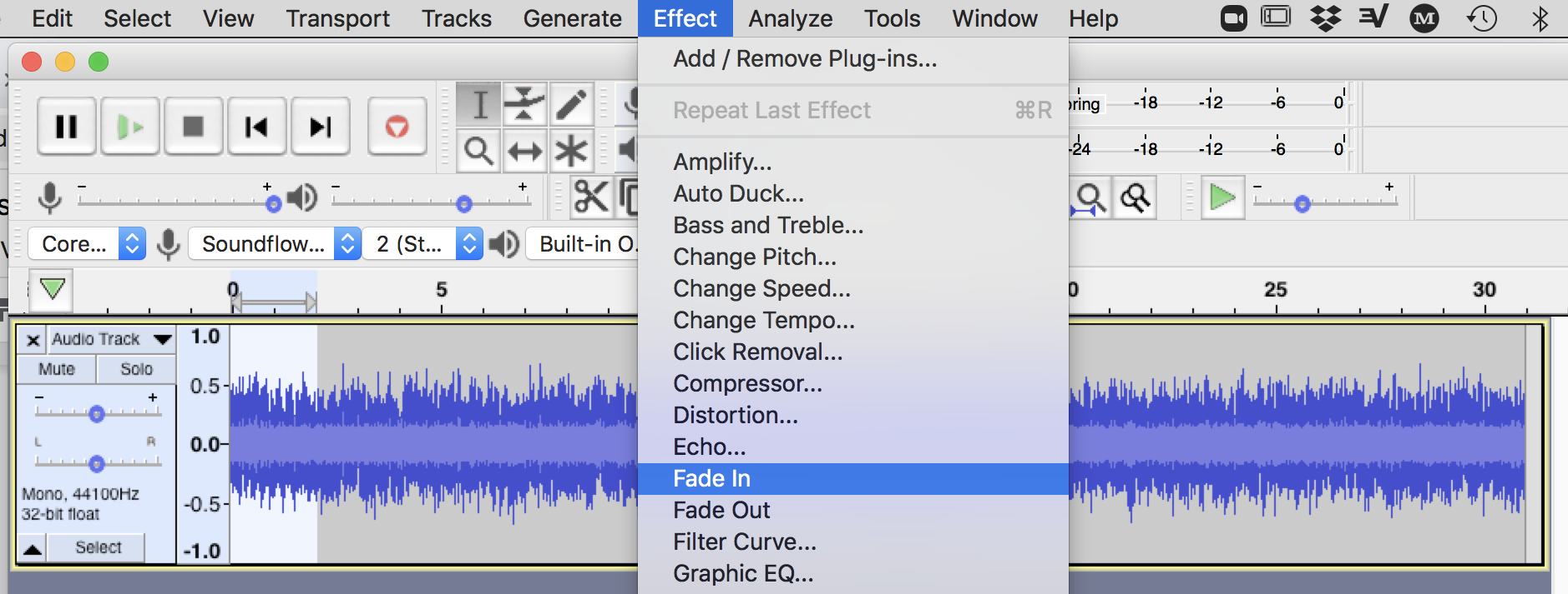
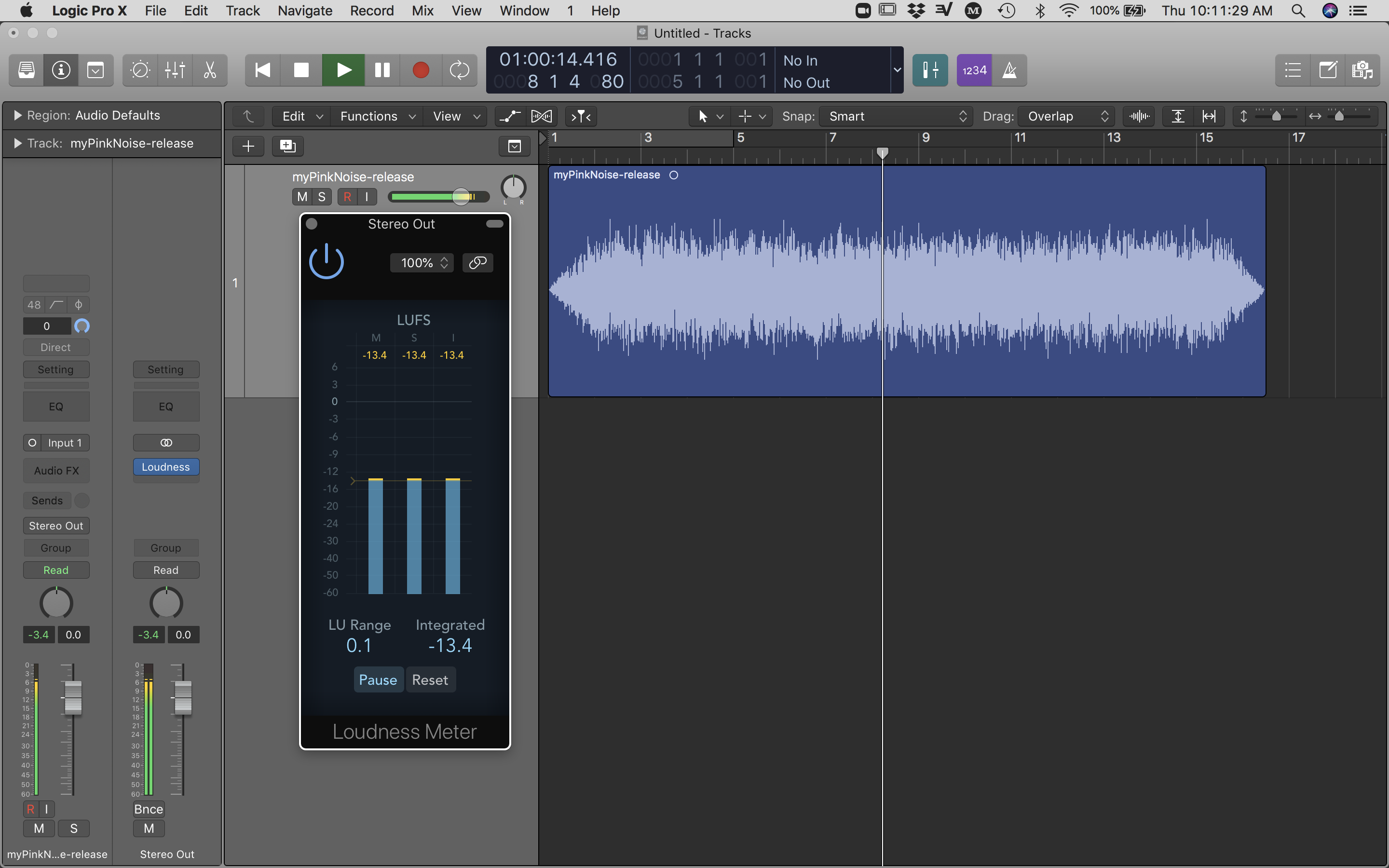
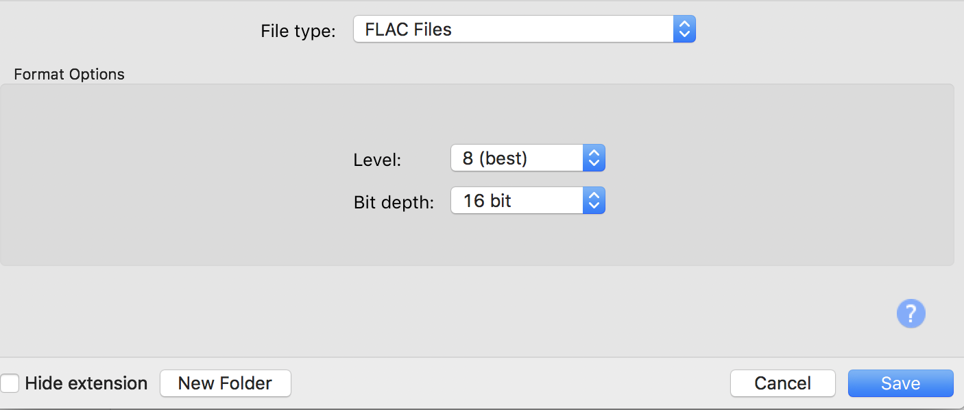
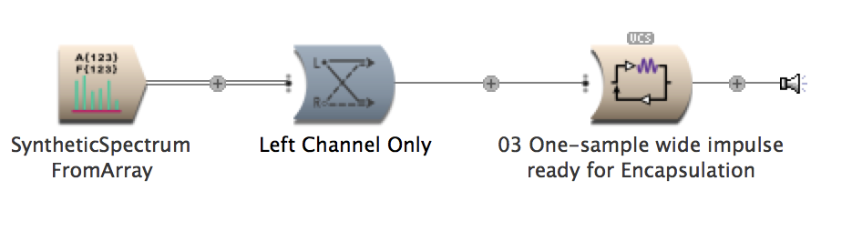
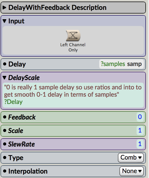
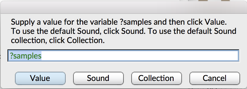
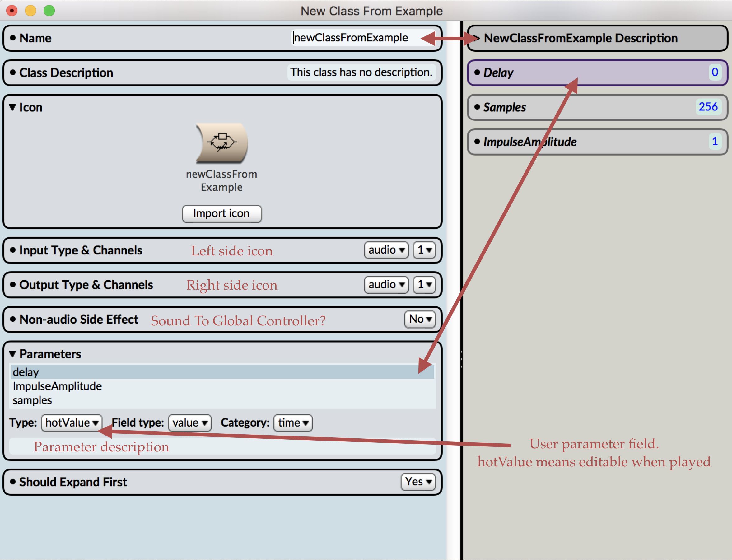
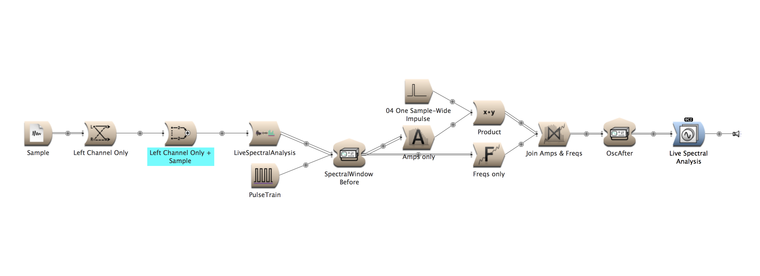
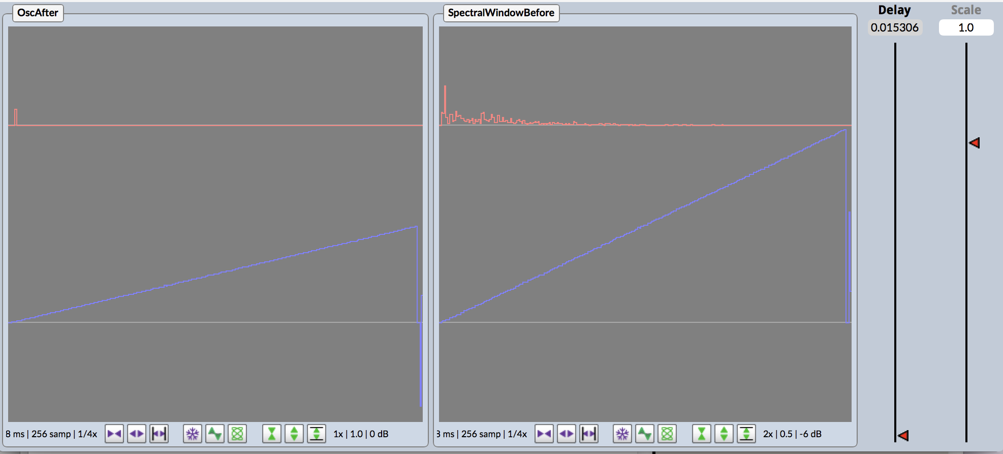
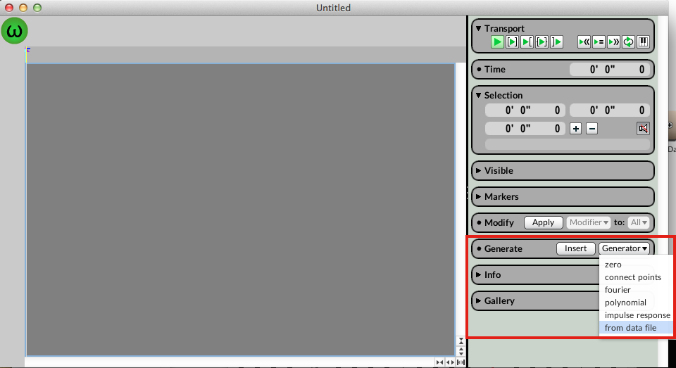
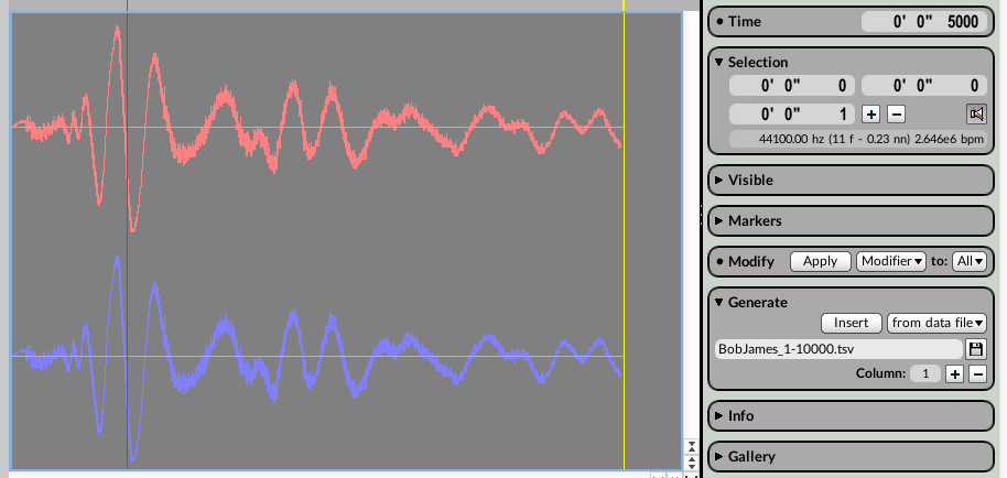
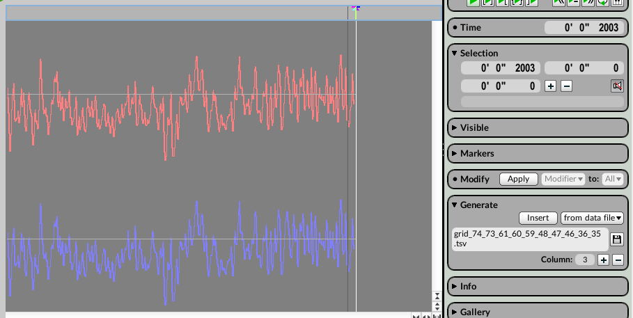
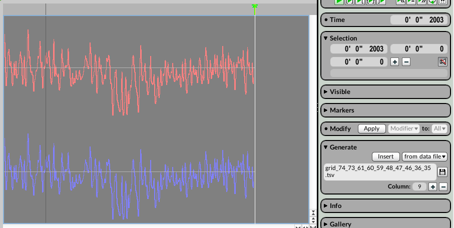
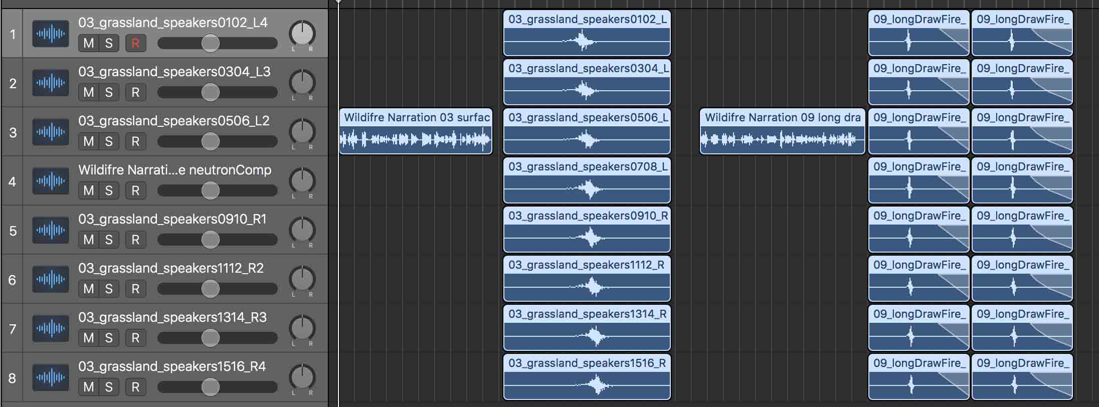
Eight different recordings of wildfire sound simulations are played across the 48-foot speaker array in looped playback. A narrator describes each wildfire event before the audio playback of fire sounds. Because audio on all eight stereo channels are triggered at the same time for simultaneous playback, audio spatialization is ‘baked-in’ on the audio files. The fire soundscapes are audio samples that have been simulated in a virtual space to move at speeds of actual wildfires and captured (read recorded) as eight stereo audio files at the same spatial location of the sixteen speakers in the physical world. The virtual mapping and recording process ensures little destructive interference as a result of phase shifts and time delays. I then mixed the resulting files inside Logic Pro X (see Figure below).
I am always amazed by how different topics are defined and vocabulary used when working across disciplines. For example, in seeking to play audio at varying rates of ‘speed,’ wildfire scientists and firefighters instead describe fires in terms of ‘rate of spread.’ Because fires are not single moving points but instead lines that can span miles moving in various directions all at once, speed is difficult for the field to put into practice. The term ‘spread’ and how it’s calculated serve wildfire science well but required me to think about how to convey the destructive ‘rates of spread’ as a rate a general observer may perceive along a two-dimensional speaker array (speakers mounted along a wall).
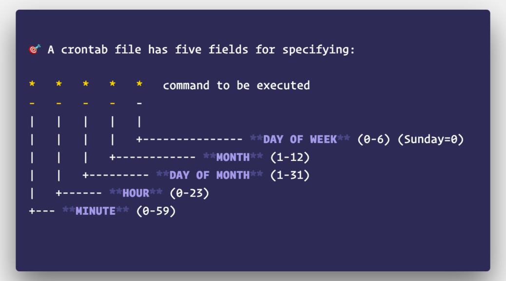
In order to distill wildfire science down to essential components for a gallery sound installation, I spent a lot of time speaking with various wildfire scientists on the phone, emailing various fire labs, working on estimating wildfire behavior using Rothermel’s Spread Rate model,[1][2] and working between the measured distance of ‘chains’ and miles. I am not a fire scientist; I am indebted to the help I received but any incongruencies are my own. I compiled eight narratives that juxtapose ‘common’ rates depicted in simulated models with real wildfires that have occurred in US western states over the past ten years based upon fire behavior (fuel, topography, and weather). These narratives are outlined in Table 1 at the bottom.
Earlier in the year, I worked with Harmonic Laboratory, the art collective I co-direct, on a 120- speaker environmental sound work called Awash.[3] The work was commissioned for the High Desert Museum in Bend, Oregon as part of the Museum’s 2019 Desert Reflections: Water Shapes the West exhibit, which ran from April 26 to Sept. 27, 2019. The 32’ x 8’ work evokes the beauty of the high desert through field recordings, timbral composition, and kinetic movement (Figure below).
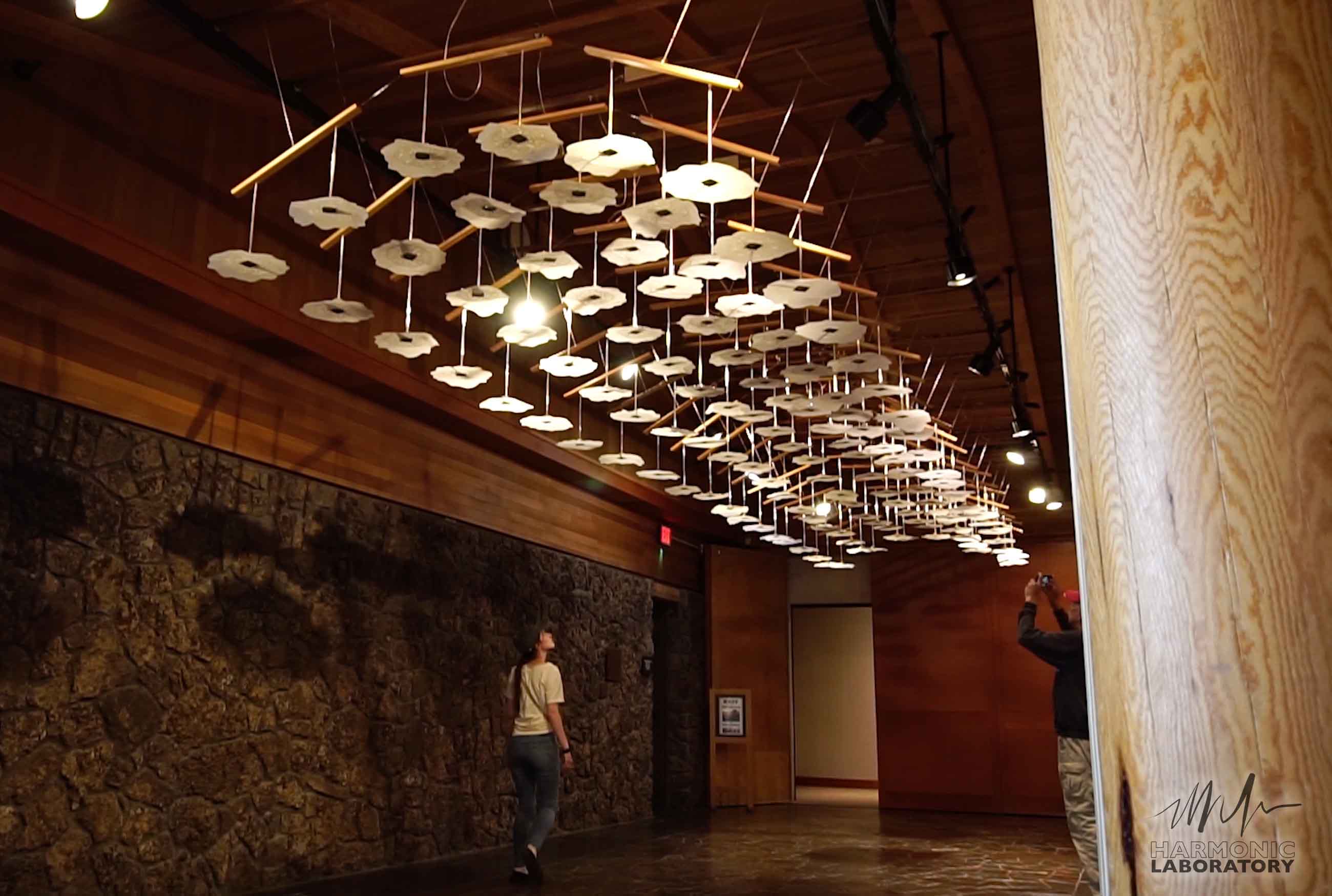
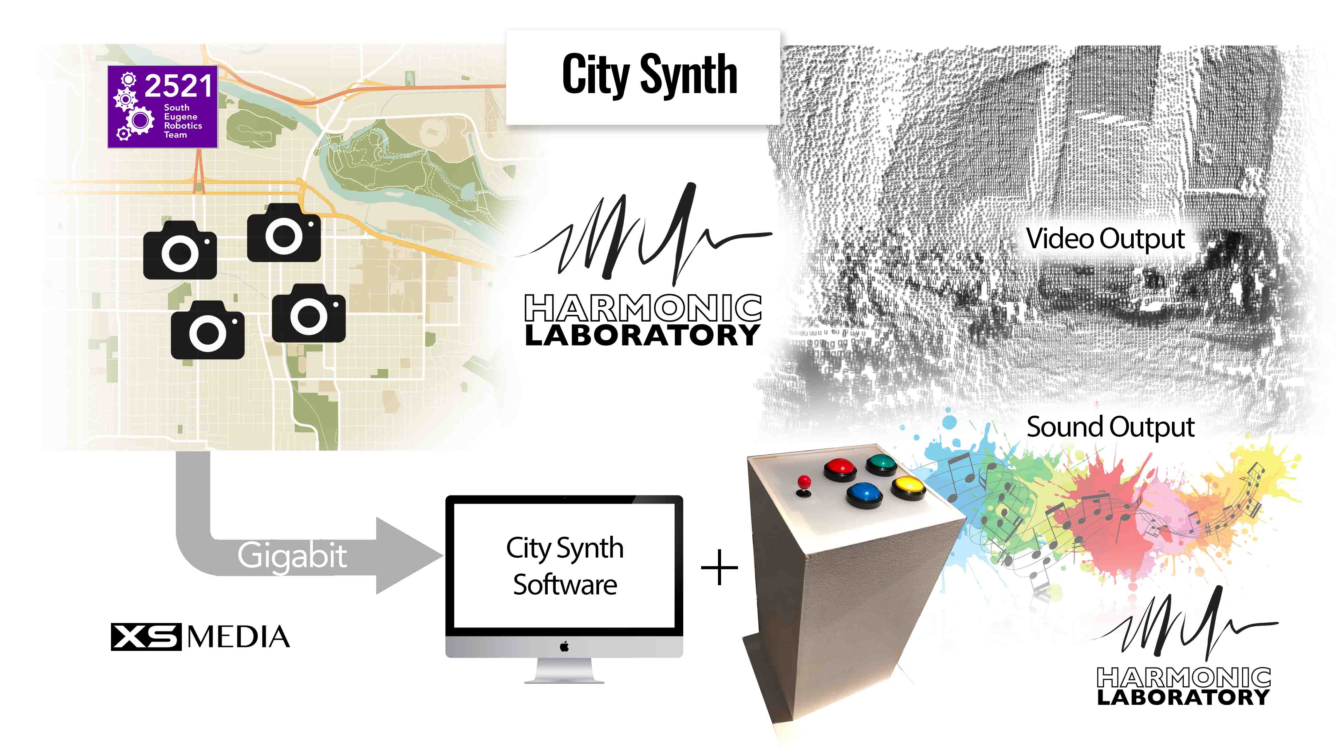
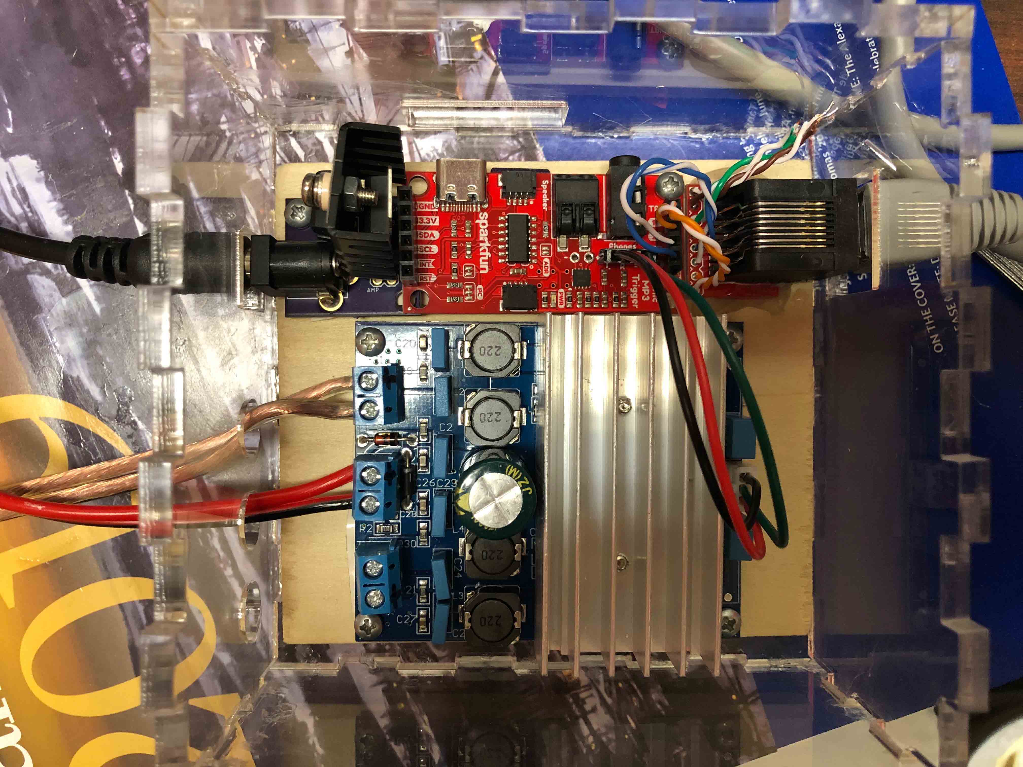
The electronic technology that I implemented in Awash for playing back audio across 120-speakers influenced my design of Wildfire. The electronics in Awash works by sending a basic low-voltage signal from the Arduino Mega motherboard to ten sound FX boards across Ethernet cable, thereby triggering simultaneous playback of audio across all 120-speakers (twelve 3W speakers per board powered by a 20W amplifier circuit). The electronics in Wildfire function in the same way: a low-voltage signal from the motherboard (Arduino Mega) is sent to eight electronic MP3 boards across Ethernet cable, thereby triggering simultaneous playback of audio across all sixteen speakers (Figures below). Instead of 3W speakers and 20W power amp boards used at the High Desert Museum, I chose to scale down the number of speakers and ramp up the wattage per board, choosing a stereo 50W power amp matched with two 30W speakers. The result is sixteen channels of audio running across eight stereo boards. And it doesn’t have to be sample-accurate!
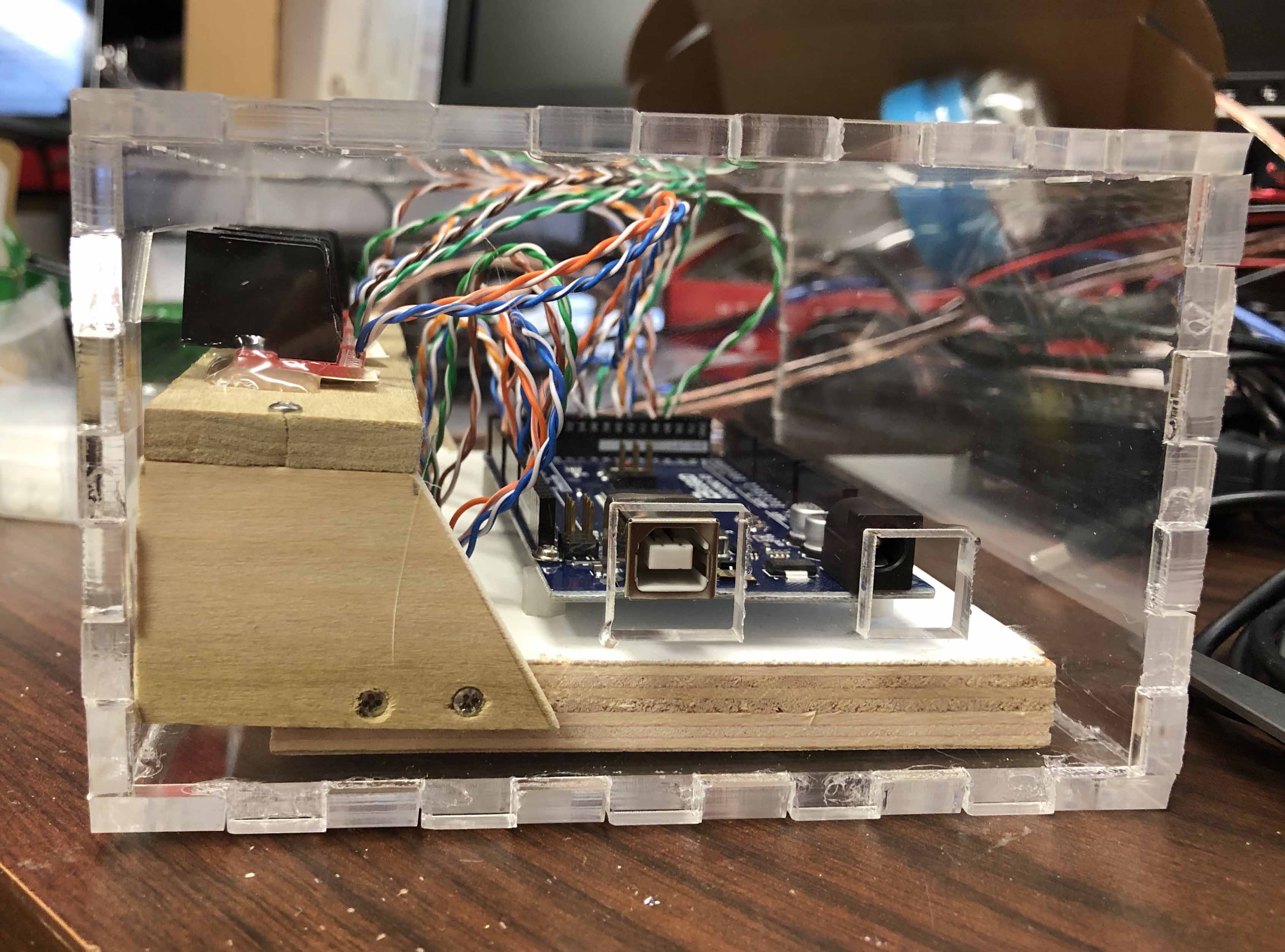
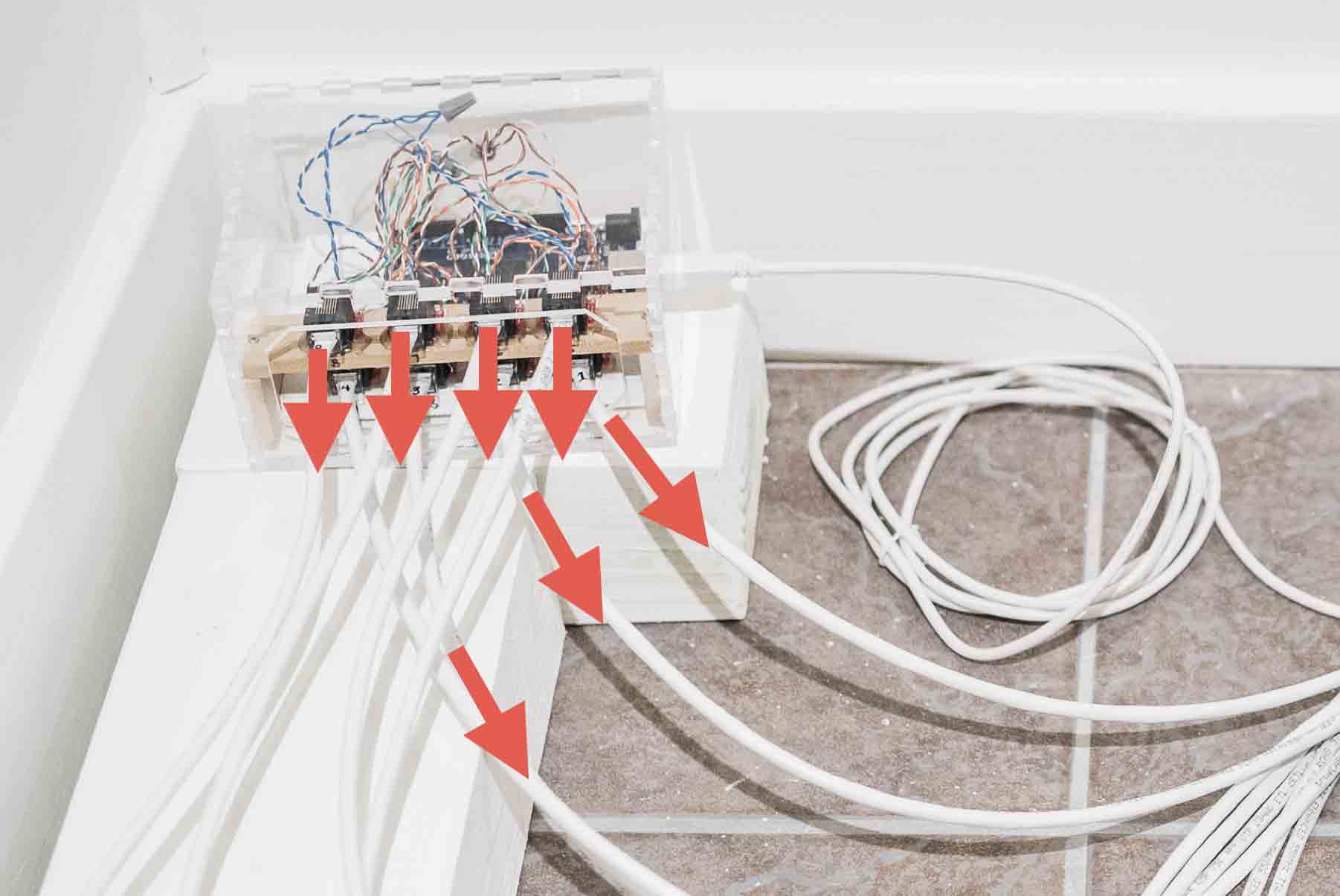
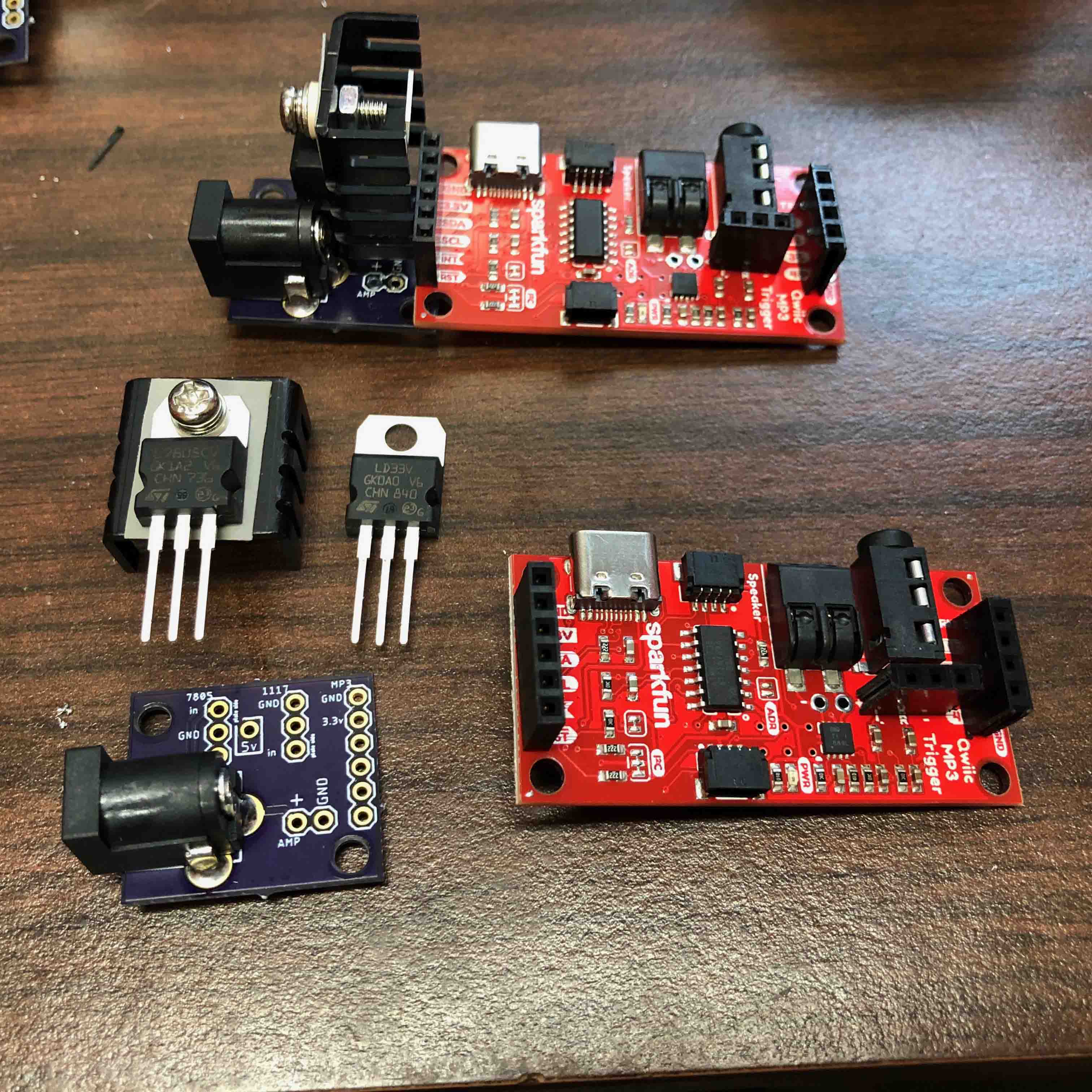
For Wildfire, I built custom laser-cut acrylic enclosures for the electronic boards (Figure below) using MakeABox.io (note: I found a good list of other services here). The second element was designing and creating custom PCB boards for the electronics themselves (Figure below). For the custom PCB board, I used Eagle CAD software (SparkFun has a great tutorial!) and then used an Oregon-based manufacturer OSH Park to print the boards.
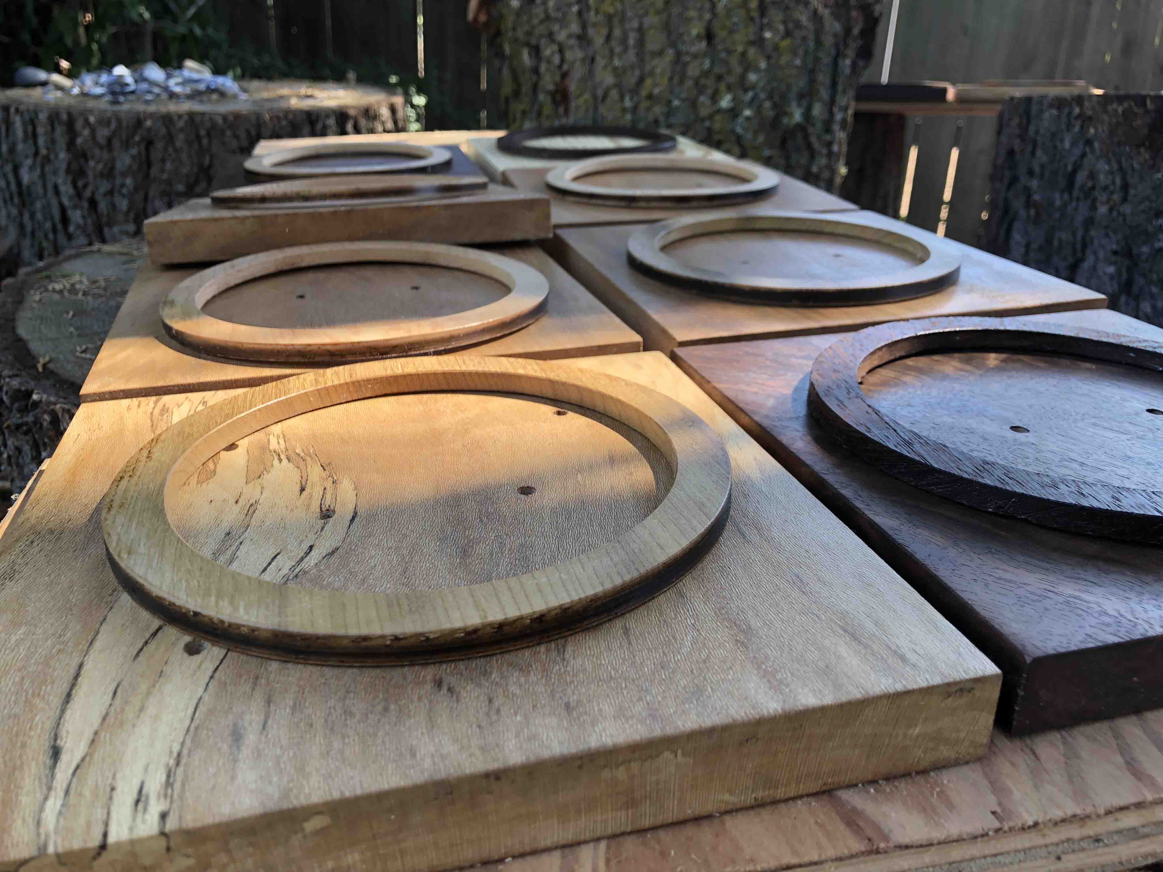
For the sixteen panel mounts and speaker rings, I sourced all wood from the woodshop at my father-in-law’s, who has various wood collected over the last 50-60 years. The panels were planed, cut, and drilled on-site and the speaker rings were cut using a drill press. The figure below depicts the raw materials after applying a basic wood varnish. The wood mounts consist of black walnut, pine, and sycamore woods. The wooden speaker rings consist of alder, ebony, and myrtle woods.
In the build-out, I was unable to power both the power amp and the MP3 audio boards from a single power source, even with voltage regulators. A large hum was evident during the split of power. A future work could attempt to power from a single power source while sharing ground with the motherboard. Yet, the audible hum led me to power the boards separately.
During install, I ran into issues of triggering related to the MP3 Qwiik trigger boards. The power draw for each MP3 board is between 3 to 3.3V, and I ran four boards from a single 9V 5A power supply using a custom T-tap connector cable and 1117 voltage regulators, in which I registered 3.26V along each power connection. However, upon sending a low-voltage trigger from the motherboard to the MP3 boards, I was unable to successfully trigger audio from the fourth and final board located at the end of the power supply connector cable. The problem remained consistent, even after switching modules, switching boards, testing Ethernet data cable, testing a different I2C communication protocol in the same configuration, among other troubleshooting tasks. When powering the final board with a different power supply (5V 2A supply), I was able to successfully trigger all eight electronic boards at once. It should be noted that the issue seems to have cascaded from my failure to effectively split power from a single power source per electronics module.

The minimal aesthetic was slightly hindered due to the amount of data and power cables running along the floor. There is minimal noise induction with long speaker cable runs, such that in my second install at SPRING|BREAK in NYC, I relied on longer speaker cable runs instead of long power and data cables. Speaker cable is cheaper than power cable, so keeping costs down, saving time in dressing cables, and minimizing cabling along the 48’ span, focusing the attention on the speakers, wood, and audio. And, if I use the MP3 boards again, I would implement the I2C protocol and consolidate the electronics, which would save on data cabling.

Through the active listening experience of hearing sounds of wildfires at realistic speeds, viewers are openly invited to support sustainable and resilient policies, including ones that can be done immediately, like creating defensible space around their homes. In the face of continued ongoing wildfires that become more frequent, Wildfire sonically strives to impact the listener in registering the devastation caused by wildfires. Getting the public to support sustainable policies and/or individually prepare for wildfires helps make communities more resilient to the impacts of wildfires and other disaster-related phenomena caused by climate change.
The work was made possible through the University of Oregon Center for Environmental Futures and the Andrew W. Mellon Foundation. The Impact! exhibition at the Barrett Art Gallery was supported with funds from the Oregon Arts Commission. Thank you to Meg Austin for inviting me to display work at the Barrett Art Gallery, and I am indebted to Sarisha Hoogheem and Matthew Klausner for their hard work in putting the show together. Thank you to Meg Austin and Ashlie Flood for curating Wildfire at SPRING|BREAK in NYC. And kudos again to Matthew Klausner and Jay Schnitt for their hard work in putting the piece up. Thank you to my cousin John Bellona, a career Nevada firefighter, for his insight on western wildfires and contacts in the field. Thank you to Dr. Mark Finney for providing common averages of speed-related to wildfires; Dr. Kara Yedinek for sharing insights on audio frequencies from her fire research; and Sherry Leis, Jennifer Crites, Janean Creighton and the other fire specialists who helped me along the way.
Table 1: Narratives in Wildfire
|
Feature |
Characteristics |
Rate of Spread |
Time across 48-foot speaker array |
|
Surface Fire: Grass Yarnell Hill Fire, June 30, 2013 Crown fire: Forest Delta Fire, near Shasta, California. September 5th, 2018 Surface Fire: Western Grassland, Short Grass Long Draw Fire. Eastern Oregon. July 12, 2012 Crown Fire: Pine and Sagebrush Camp Fire, near Paradise California. November 8th 2018. |
Low dead fuel moisture content, High wind speed, Level terrain 3-6% dead fuel moisture content, Wind speed 15-25 mph, Mixed terrain Low dead fuel moisture content, High Wind speed, Level terrain Moisture content unknown, Wind speed unknown, Mixed terrain 2% Dead Fuel Moisture, Wind speed 20 mph, Level Terrain Moisture content unknown, Wind speed unknown, Mixed terrain 2% Dead Fuel Moisture, Wind speed 20 mph, Level Terrain Low Moisture content, Wind speed 50 mph, Mixed terrain |
Upper average forward rate of spread, 894 chains/hour During Granite Mountain crew de- ployment, 1280 chains/hour Upper average forward rate of spread, 297.6 chains/hour Initial perimeter rate of spread, 16,993 sq. chains/hour Perimeter rate of spread, 1250 chains/hour Average perimeter rate of spread, 61,960 sq chains/hour Perimeter rate of spread 525 chains/hour Peak perimeter rate of spread, 67,000 sq. chains/hour |
2.92 seconds 2.04 seconds 8.7 seconds 1.54 seconds 2.16 seconds 0.422 seconds 4.99 seconds 0.394 seconds |
[1] F. A. Albini, “Estimating wildfire behavior and effects,” United States Department of Agriculture, Forest Service, Tech. Rep., 1976.
[2] J.H. Scott and R.E. Burgan, “Standard fire behavior fuel models: A comprehensive set for use with Rothermel’s surface fire spread model,” United States Department of Agriculture, Forest Service, Tech. Rep., June 2005.
[3] J. Bellona, J. Park, and J. Schropp, “Awash,” https://harmoniclab.org/portfolio/awash/