Over the summer, I produced five sound sculptures centered around fire-affected areas of the 2020 Holiday Farm fire. The work was part of the Soundscapes of Socioecological Succession (SSS) project that was funded through a Center for Environmental Futures, Andrew W. Mellon 2021 Summer Faculty Research Award from the University of Oregon.

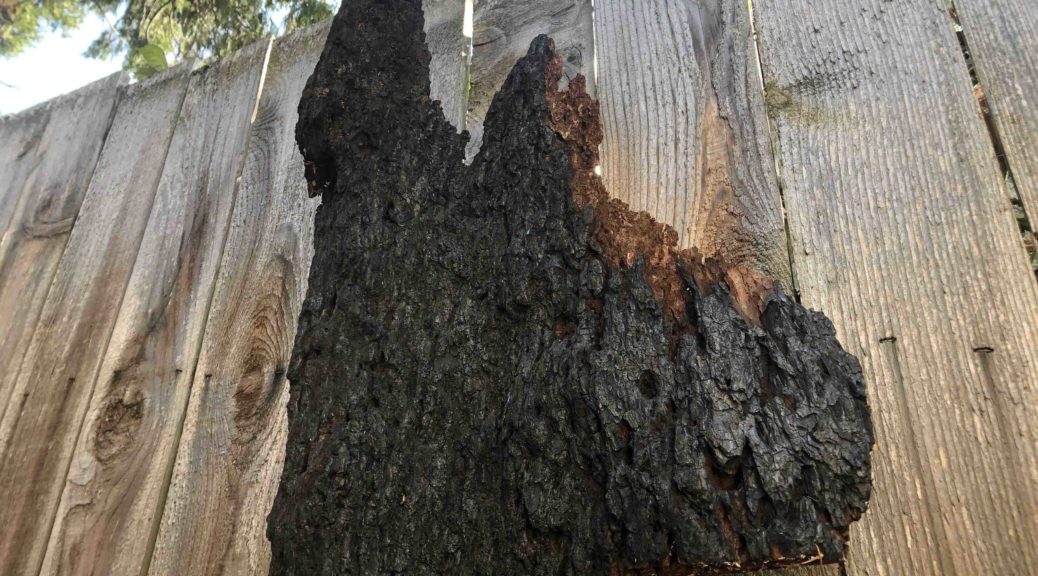
Through field recording fieldwork, local wood sourcing, and custom electronic design, the five (5) sound sculpture prototypes were one way to generate a unique auditory experience aimed at the general public. The work was designed to unpack the sounds and scenes of wildfires in natural and human-systems and to document the regenerative succession of coupled social and ecological processes.

Video 1. Sound sculpture C prototype. Burnt cedar wood and audio sourced from fire affected area near Blue River, OR.

Socioecological systems emerge from interdependent processes through which people and nature self-organize across space and time (Gunderson and Holling, 2002). STEM-centric studies of socioecological dynamics miss literal and metaphorical connections between people and nature, which are difficult to quantify and to communicate. To address this limitation, the sound sculptures test a new approach to capture SSS as a qualitative record of collective response to catastrophic wildfire.

Like a slice of tree ring that marks age and time, the field recordings of audio in visits to fire-affected areas connotes a slice of succession activities. Sound recordings of the area are meant to capture multiple scenes and ecological voices, filtered through a raw material from the sites themselves.

Video 2. Sound sculpture D prototype. Wood and audio sourced from fire affected area near Blue River, OR.

Our sonic environment is polluted by man both in its content and its reflections. This is certainly true even for field recordists who venture further and further into the wild to break free from the noise pollution of a passing airplane, a highway’s din, or even audible underground activity such as fracking (One Square Inch, 2021). Treating site-specific wood as an acoustic resonator — a filter that distorts as much as it renders sound audible — casts a shadow onto the sounds it projects. The physical material acts as a filter upon the sound. The wood slightly changes the spectrum of sound by boosting or cutting the amount of different frequencies in the sound.

Our University of Oregon team expanded previous research by sampling the rich SSS at fire-affected sites, including soundscape field recordings, recorded interviews, and collecting “hazard tree” waste material. These materials offer a document of the resiliency of the landscape and illustrate how forest disturbance can set back human-defined sustainable development goals regionally. The development of the five sound sculptures are just one means to inform the public and inspire collective action towards sustainable futures.

Video 3. Sound sculpture E prototype. Wood and audio sourced from fire-affected area near Blue River, OR.

Audio field recordings were captured during two site visits to fire-affected areas on June 16, 2021 and July 2, 2021. The second visit was to H.J. Andrews forest and an interview and tour with Mark Schulze (H.J. Andrews Experimental Forest Director) Bailey Hilgren and I used a few field recording setups, and which mostly consisted of Bailey recording with a Zoom H6 using on-board mics and I recording with a Sound Devices 633 field mixer and three mics: Sennheiser MKH 30-P48 and MKH 50-P48 microphone in mid-side configuration and a LOM Uši Pro omnidirectional microphone. The Zoom recordings were captured at 96k-24bit, and the 633 recordings were captured at 192k-24bit. During the second visit, we were able to setup “tree ears” that consisted of two Uši Pro mics taped to a tree and a LOM Geofón low frequency microphone, and which we left recording for several hours in the H.J. Andrews forest (see Figure 2). Bailey organized all the audio recordings using the Universal Category System (UCS). The system is a public domain initiative for the classification of sound effects. While we chose not to make the 30+GB of audio files as a publicly available archive, we have made the audio categorization spreadsheet publicly available (SSS metadata spreadsheet).

Figure 1. Field recording setup at fire affected site.

Figure 2. “Tree ear” field recording configuration.

During the technical design phase, some secondary research questions were asked. Which audio exciter/transducers work best on non-flat, raw wood surfaces? Which exciters are the most cost-effective solution for an array of speakers?  For fabrication of installing wood as pieces on a wall, can I cost-effectively source sturdier materials than aluminum posts?

Figure 3. Sound sculpture prototypes depicting standoffs and speakers.

I tested a few different models: waterproof transducer, round and square exciters, and distributed mode loudspeakers. I also tested different speaker formats: 10W 8ohm, 20W 4ohm, and 20W 8ohm. Unfortunately, the desired power outputs, 25-30W, models of exciters were consistently sold out throughout the project, therefore I was unable to equally distribute testing across similar power outputs. From experience more than a scientific A/B test, I found that the more flexible options for attaching to wood surfaces were the Dayton Audio DAEX25Q-4 Quad Feet 25mm and the Dayton Audio DAEX32SQ-8 Square Frame 32mm Exciter, 10W 8 Ohm. Generally, I realized that in order to get decent output in both frequency response and gain, the low-end of $15-20/transducer seems about right. I do not recommend anything below 10W for this type of work. Getting a stereo image was not important and would be difficult given the size of wooden pieces. I valued volume and minimizing visual distraction, so speakers were meant to be placed behind or under the sculptures. I doubled speakers whenever I used 10W drivers.

Figure 4. Recording log loader moving hazard tree material

Audio 1. Log loader field recording (see Figure 4)

For standoffs, I sourced variable size stainless steel standoff screws used in mounting glass hardware which worked extremely well on the river wood sound sculpture (Figure 5).

Figure 5. Stainless steel standoffs, 10W 8ohm speakers, and custom electronics board on sound sculpture D prototype.

I sourced audio amplifiers on sale for under $10 each, where $15 is normal pricing. The TPA3116D2 2x50W Class D stereo amplifier boards have handled well on previous projects, and finding them cheaply with the added volume control and power switch were a great addition for fine-tuning amplification in public spaces.

Normally powering the amplifiers and audio boards is where the real cost comes in, and I was happy to learn that Sparkfun’s Redbaord Arduino’s can now handle upwards of 15VDC, so I went with their MP3 Player Shield and Redboard UNO in order to split VDC power between the amplifier and board (12V, 2A power supplies were adequate for the project and transducer wattage).

Figure 6. Custom electronics board consisting of MP3 player shield, Arduino UNO Redboard, 2x50W class D amplifier, and power split for up to 15VDC.

Figure 7. Recording site near Eagle Rock along the McKenzie River.

I modified the outdated MP3 player code on Arduino to dynamically handle any number of tracks and named audio files, such that one doesn’t need to rename audio files in the convention “track001.mp3” “track002.mp3”.  Whatever audio files are uploaded onto the SD cards, the filenames simply need to be placed into an array at the top of the code uploaded to the board. Thus, when powered on, the sound sculpture will play an endless loop of the uploaded audio files found on the SD card.

***For those interested in the Arduino code running on the MP3 players, I have made the code publicly accessible as a repository on Github.

Figure 8. Full electronics module example: 12V 2A power supply, MP3 player shield, Sparkfun Redboard Arduino, TDA 2x50W stereo amplifier, single 10W exciter.

Video 4. Sound sculpture A prototype. Wood and audio sourced from fire-affected area near Blue River, OR.

Selecting the audio for sound sculptures came through discussions with Bailey around ecological succession, the interviews conducted, and the types of audio that was captured and categorized. We chose four audio bins (categories) to work with: animals, soundscape or ambient, logging or construction, and scientific or interviews. Again, Bailey created a categorical spreadsheet of audio files within these four bins.

Video 5. Sound sculpture A prototype. Wood and audio sourced from fire-affected area near Blue River, OR.

Constructing the sound sculptures involved imagining public space and the materials. There are two pieces for wall, one for hanging, one for a pedestal, and one for the ground. The sculptures are stand alone pieces that simply require AC power for showing. See below for a gallery of stills of these works.